Comparing Activation Functions via Accuracy of Classification Neural Networks
Arnaav S. Goyal
Enloe High School
AP Statistics 1B
Mrs. Celia Rowland
May 14, 2021
Abstract
Classification neural networks can learn to classify things through stochastic gradient descent and the backpropagation algorithm. A vital part of this algorithm is the chosen activation function. This study analyzes the accuracy of three activation functions, Swish, Sigmoid, and Rectified Linear Unit (ReLU) and compares them to determine the most accurate one to use in a classification neural network. Accuracy data was collected on 300 classification neural networks (n = 100 for each function), trained over 60,000 images and tested over 10,000 images from the MNIST database. The ReLU function is found to be more accurate than the Sigmoid, and the Swish function is found to be more accurate than the ReLU.
Introduction
Classification neural networks (CNNs) are used broadly in today’s world, in everything from search engines to artificial intelligence. They are structured as layers of neurons, with each successive layer’s neurons connecting to every neuron in the previous layer with a unique set of weights. Each neuron also has a bias associated with it. Both the weights and biases are numbers that weigh the previous neurons’ values and bias[1] the result, respectively, and are the basis of neuron calculations (see fig. 1). A big part of these calculations are the activation functions used in each neuron of the network. Activation functions take the previous activations (if applicable), weights, and bias and scale them as one value that acts as the neuron’s activation. Activation functions must fulfill many conditions to work in a neural network, and the specific function used can greatly influence the accuracy of the neural network. Here, we focus on and compare the accuracy of three popular activation functions: Swish, Sigmoid, and Rectified Linear Unit (ReLU). We hypothesize that Swish will come out on top due to how well it combines the strengths of both ReLU and Sigmoid.
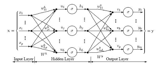
Figure 1
Diagram of a Simple Neural Network
Note. Each value shown has index notation to represent which layer and neuron it belongs to. The weights are represented by w, and every weight is represented by a connecting line between neurons of consecutive layers. The total input value is shown as u, the activation function is shown as 𝜎, and the activation value is represented with h.
Method
Neural network learning
A method called stochastic gradient descent was used to train the neural networks using the backpropagation algorithm. This algorithm involves starting from the output layer and working backwards to calculate the loss function of the network. The loss function is an n-dimensional function that graphs the loss of the network as a whole, where n is the total number of weights and biases used. The algorithm then descends the loss function gradient by changing the weights and biases, minimizing the loss function and therefore making the network more accurate. Activation functions play a large role here, as the derivative of the activation function is used to calculate the loss function and descend the gradient.
Batch learning was utilized in conjunction with stochastic gradient descent for training the neural networks. This means that for every b inputs processed through a neural network, where b is known as the batch size, backpropagation was performed once. Training sets are finite, so training a neural network usually involves iterating over the entire training set multiple times. Each iteration over the set is called an epoch. For example, you could train a network for 3 epochs over a training set of 600 data with a batch size of 10.
Procedure
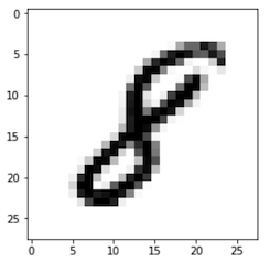
The MNIST database provides 70,000 classified 28x28 pixel grayscale images that represent numbers (fig. 2). Using MNIST, 300 CNNs were trained for 5 epochs over a training set of 60,000 images with a batch size of 30. Each network’s weights and biases were initialized with random numbers between -1 and 1. 100 networks used Sigmoid for their activation function, 100 used ReLU, and the last 100 used Swish. The networks were then tested on a test set of 10,000 images, and their percentage accuracies were recorded in a Google Sheets.
Figure 2
Example of an Image from the MNIST Database
Note. This image represents an 8, so the neural network would be expected to respond with an 8.
Activation function definitions
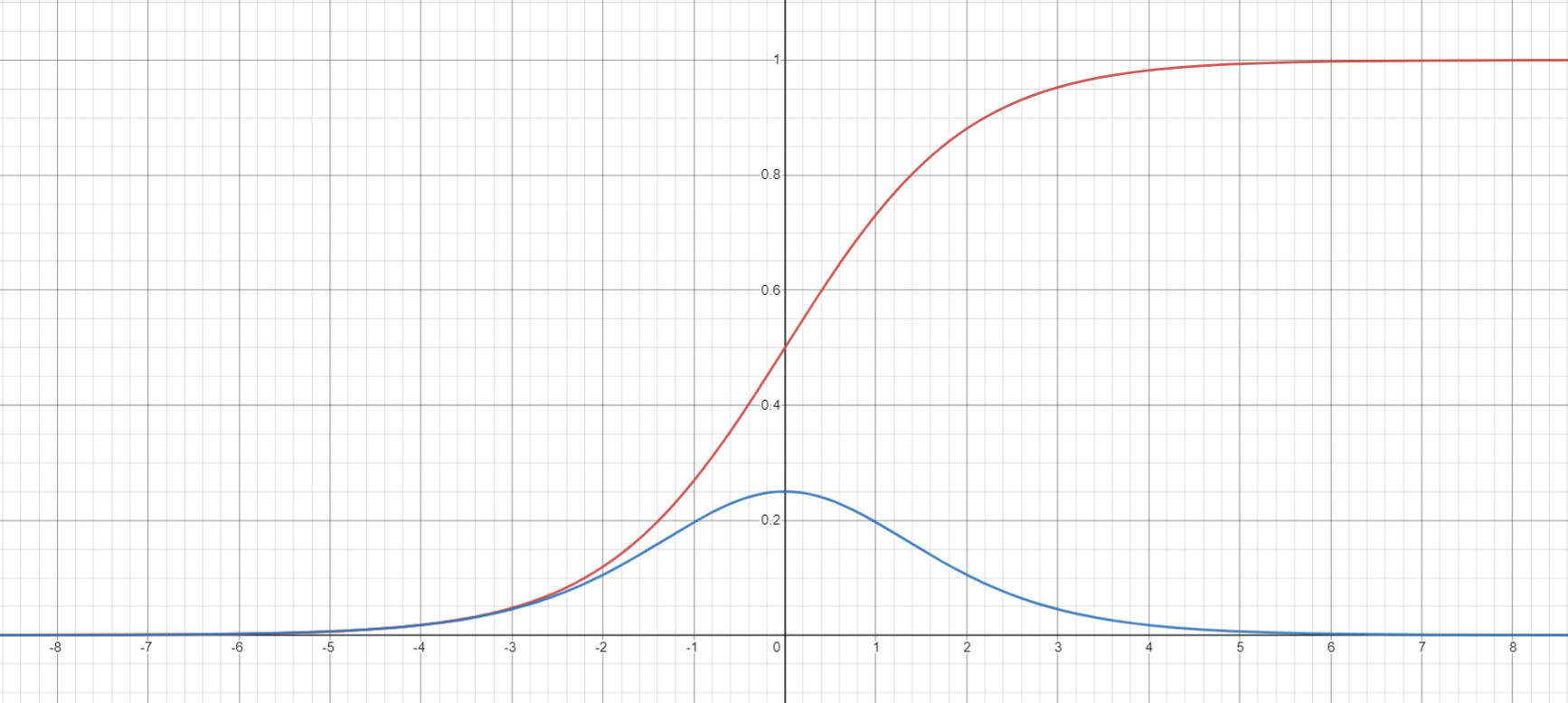
Sigmoid is defined as  , and its derivative, in the form used in the program, is
  (fig. 3). ReLU is defined as
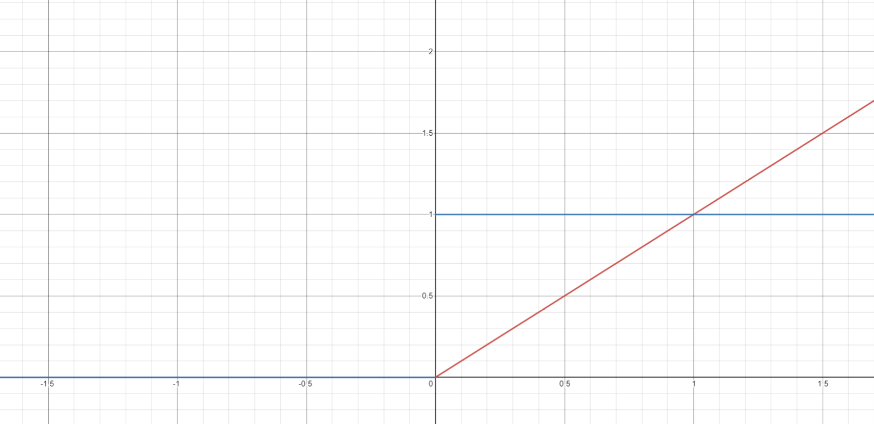
  and its derivative is
  , where
  is the Heaviside step function (fig. 4). Swish, in the program, is defined as
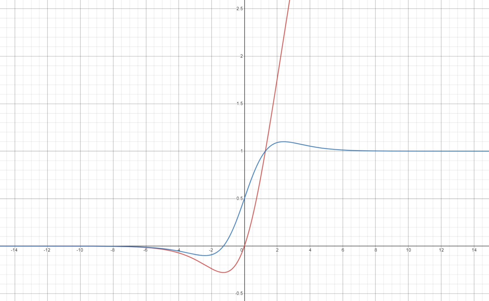
  , and its derivative is
  (fig. 5). There is sometimes a
  term added, but it was not needed for our purposes. Notice how every one of these functions approach 0 when going to -∞.
Figure 3
Graph of the Sigmoid Function and its Derivative
Note. The Sigmoid function is graphed in red, and its derivative is graphed in blue. The graphs overlap in the approximate range  .
.
Figure 4
Graph of the ReLU Function and its Derivative
Note. The ReLU function is graphed in red, and the derivative is graphed in blue. The graphs overlap in the approximate range  .
.
Figure 5
Graph of the Swish Function and its Derivative
Note. The Swish function is in red, and its derivative is in blue. The graphs overlap in the approximate range  .
.
Neural network architecture
The neural networks created all had the same architecture: 3 layers, with 784 neurons in the input layer, 128 neurons in the hidden layer, and 10 neurons in the output layer. Therefore, the loss function for the networks was in 101,770 dimensions (101,632 weights and 138 biases). The activations for each of the 784 neurons in the input layer were the scaled pixel values of the image, flattened left-to-right, top-to-bottom. For example, the activation of the 31st neuron in the input layer would be set to the value of the 3rd pixel in the 2nd row of the input image. The values from the MNIST database range from 0 (black) to 255 (white), so they were divided by 255 to scale the pixel values between 0 (black) and 1 (white). The hidden layer and output neurons used the formula  to determine their activations, where i is the current layer, j is the current neuron in layer i, ni is the last neuron in the i-th layer,
  is the weight between the m-th neuron in the i-1 layer and the j-th neuron in the i-th layer, and
  is the bias of the j-th neuron in the i-th layer. The activations of the output layer were then used to determine the result. For example, if the network outputted [0: 0.0052, 1: 0.0023, 2: 0.0601, 3: 0.0065, 4: 0.0396, 5: 0.0001, 6: 0.0385, 7: 0.0046, 8: 0.8429, 9: 0.0002], its result is 8, since the value at position 8 is substantially greater than the rest.
Results
Data and distributions
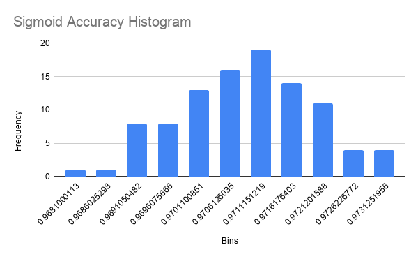
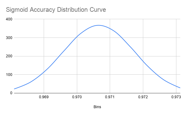
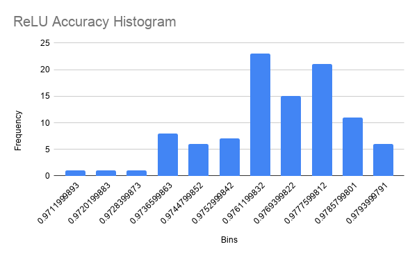
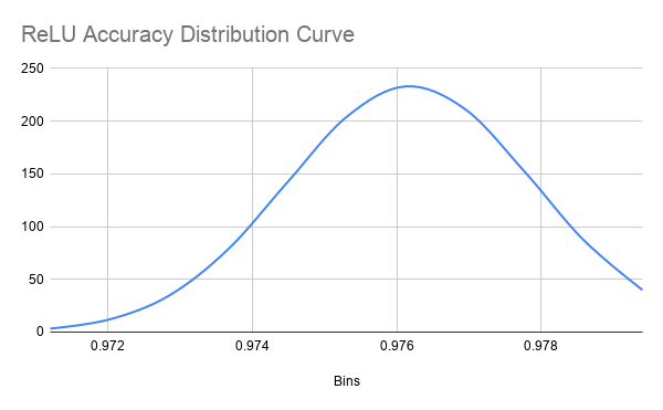
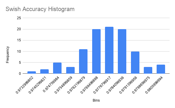
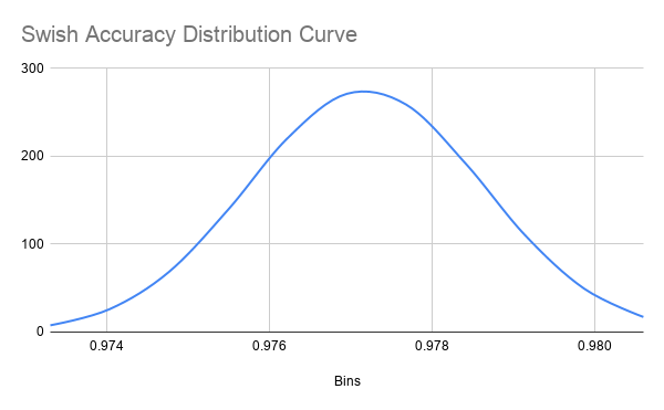
One data point in the Sigmoid accuracies was an outlier (less than 1st quartile minus 1.5 times IQR). I suspect that this was because the backpropagation algorithm descended the gradient into a local minima rather than an absolute minima. This is only possible because of random initialization and cannot be avoided. I feel this renders the data point irrelevant to the distribution because it is not representative of the accuracy of the network. The mean accuracy for networks using Sigmoid, ReLU, and Swish as their activation functions was 0.9706656584 (SD = 0.001086108654), 0.9761869991 (SD = 0.001710729488), and 0.9771810001 (SD = 0.001452597078), respectively. The distribution of accuracy for Sigmoid networks is perfectly bell-shaped but very wide, so we can approximate it to a t-distribution (fig. 6 and 7). The distribution of accuracy for ReLU networks is left skewed as well, and is also slightly wider, but still resembles a bell curve and can be approximated to a t-distribution (fig. 8 and 9). The accuracy distribution for Swish networks is wide but not very skewed, resembling a bell curve very well, so it can be approximated to a t-distribution. (fig. 10 and 11).
Figure 6
Histogram for Sigmoid Network Accuracy
Figure 7
Distribution Curve for Sigmoid Network Accuracy
Figure 8
Histogram for ReLU Network Accuracy
Figure 9
Distribution Curve for ReLU Network Accuracy
Figure 10
Histogram for Swish Network Accuracy
Figure 11
Distribution Curve for Swish Network Accuracy
The conditions for both two-sample t-tests conducted later to compare the accuracies are fulfilled as follows:
We define the parameters for the first two-sample t-test as such: the population of ReLU CNNs 𝜇R, the population of Sigmoid CNNs 𝜇S, and the significance level 𝛼 = 0.01. We define the hypotheses to be H0: 𝜇R - 𝜇S = 0 and HA: 𝜇R - 𝜇S > 0. We obtain a test statistic of t = 26.96980143, with a p-value of p = 0. Because p < 𝛼, we reject H0. Therefore, we have significant evidence to state that ReLU CNNs are more accurate than Sigmoid CNNs.
Using the results from the previous test, we compare ReLU network and Swish network accuracy. We define the parameters to be the population of Swish CNNs 𝜇S, the population of ReLU CNNs 𝜇R, and the significance level 𝛼 = 0.01. The hypotheses are defined as H0: 𝜇S - 𝜇R = 0 and HA: 𝜇S - 𝜇R > 0. We obtain a test statistic of 4.429111906, with a p-value of 0.000007818631021. Because p < 𝛼, we reject H0. Thus, we have significant evidence that Swish CNNs are more accurate than ReLU CNNs. These results support our hypothesis that Swish CNNs are the most accurate amongst the three compared. However, it was unexpected that ReLU and Swish were so close, while Sigmoid fell so far behind.
Considerations
Architecture limitations
Because of the infinite possibilities of CNNs, the scope of these findings is very limited. CNNs can have significantly more neurons than the architecture we used here, in which case the exploding gradient problem comes into play. The exploding gradient problem is when the activation values of neurons grow much too large and the network outputs nonsense. When you have a large number of neurons, you add more and more values per activation, which will lead to “exploding” values. Sigmoid counters this problem significantly better than both ReLU and Swish because it is essentially bounded between 0 and 1 on the y-axis, while both ReLU and Swish grow infinitely. Therefore, if you have a CNN with many neurons, Sigmoid may be the best activation function.
Another such problem is the vanishing gradient problem. This occurs when you have a CNN with many more hidden layers than what we used here. Backpropagation iterates through the layers multiplying derivatives with each other, so with many layers and small derivatives (less than 1), backpropagation will multiply many small numbers with each other. This will make your gradient descent values so incredibly small that your gradient essentially vanishes, making your network useless. Both ReLU and Swish counter this problem because their derivative can be larger than 1. Swish is especially good because its derivative can be anything between -0.0998 and 1.0998, while still being bounded between 0 and 1 for large values. However, Sigmoid’s derivative will always be under 1, meaning that a network with more than just a few layers using Sigmoid will be susceptible to the vanishing gradient problem.
Dead neurons are yet another problem. Since backpropagation relies on multiplication, if a value is ever set to zero, it will usually be stuck at zero. ReLU networks are especially susceptible to this, as any value below 0 will automatically be set to 0 with both ReLU and its derivative. Swish and Sigmoid are not as susceptible because they have smooth curves that approach zero asymptotically. This means that neurons will never be set to 0 - with the exception of extreme values like 10,000, but in that case you probably have an exploding gradient problem - so they can always be recovered by the backpropagation algorithm.
Pseudo-randomness
No computer program can ever generate a truly random number, meaning that the weights and biases are pseudo-random. This is worth consideration considering the sheer amount of random values being initialized in my samples. For reference, there were 101,770 values initialized per network, for a total of 30,531,000 pseudo-random numbers generated.
Type of neural network
The type of neural network is vitally important in deciding which activation function to use. For this experiment, we used a classification neural network intended to classify images as numbers. However, there are other types that don’t classify. For example, some neural networks can dynamically identify sentences from audio. The requirements and calculations involved in these networks are vastly different from the ones used in our networks. Therefore, the results of accuracy we have found here are not at all applicable to other types of neural networks like those.
[1] Note: the term bias used here is not to be confused with statistical bias. Here, bias simply means that the value is used to move the result of a neuron’s calculation a specific way, determined by the learning algorithm.